Introduction
Estimating depth using images from two cameras that are a fixed distance appart is a technique known as stereo vision or stereo depth estimation. It mimics how human eyes perceive depth by using the slight difference (disparity) between two images captured from slightly different viewpoints. The process involves capturing images, rectifying them to align corresponding points, matching features between the images, and computing disparity. Depth is then derived using the formula $$Z = \frac{f⋅B}{d}$$ where Z is depth, f is focal length, B is baseline distance between the cameras, and d is disparity. The result is a depth map, where each pixel represents the distance to objects in the scene. Monocular depth estimation is the process of determining the distance and depth information of objects in a scene using a single image, as opposed to relying on stereo or multiple camera setups. It involves the use of advanced algorithms and deep learning techniques to infer the three-dimensional structure of a scene from two-dimensional images captured by a single camera. Despite the rapid development in deep learning techniques, estimating depth using stereo vision is still more reliable for self-driving cars.
Basics problem statement
This work builds upon the work done by Kim et al. in their paper "SimVODIS: Simultaneous Visual Odometry, Object Detection, and Instance Segmentation".
SimVODIS is designed to extract both geometric features (such and pose estimation and depth map prediction) and semantic featrues (such as object detection and instance segmetntaion)
from a sequence of image frames. Instead of using image from multiple sets of cameras this approach works with a sequence onf images from the same camera \((I_{t-1}, T_t)\). Imagine the following motion vector:
$$u_{target, source} = [t^T, r^T]^T$$
which is used to generate a certain target if source, the translation vector \(t = [\Delta x, \Delta y, \Delta z]^T\) and the rotation vector \(r = [\Delta \theta, \Delta \phi, \Delta \psi]\). The main goal of the architecture is to maximize the conditional probability of the motion vector \(u_{target, source}\) and the depth \(D_t\)
$$\dot{u}_{t, t-1}, \dot{D}_t = argmax_{u_{t, t-1}, D_t} P(u_{t, t-1}, D_t | I_t, I_{t-1})$$
when the sequence of monocular images \((I_{t-1}, I_t)\) at time step t. This conditional probability can be further expanded as follows:
$$P(u_{t, t-1}, D_t | I_t, I_{t-1}) = P(u_{t, t-1} | I_t, I_{t-1}) . P(D_t | I_t, I_{t-1})$$
$$P(u_{t, t-1}, D_t | I_t, I_{t-1}) = P(u_{t, t-1} | I_t, I_{t-1}) . P(D_t | I_t)$$
SimVODIS used 3 consecutive images when estimating motion vectors for a more robust performance, this modifies the above equation as follows:
$$\dot{U}_{t}, \dot{D}_t = argmax_{(U_{t}, D_{t})} P(U_t | I_{t+1},, I_t, I_{t-1}) . P(D_t|I_t) $$
where \(U_t = [u_{t,t-1} ; u_{t, t+1}]\) which just means that the image at time \(t\) will once be generated using the image at time \(t-1\) and once using image at time \(t+1\).
The simplified version of the network used to predict the depth and motion vector is shown in the image below.
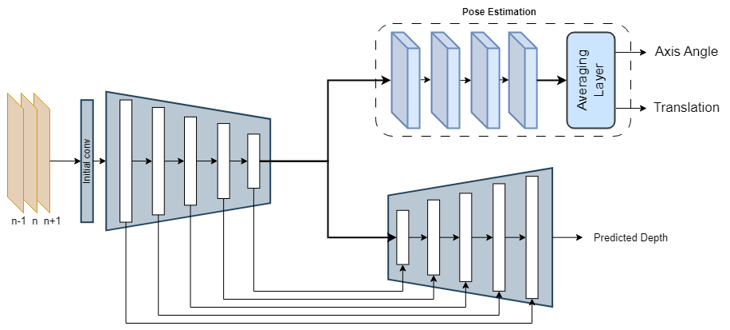
The network has a single encoder, a pose estimation branch and a depth estimation branch. The pose estimation branch. During the training process the network searches and learns optimal parameters for depth and pose estimation branches to maximize the conditional probability shown above. This training process works by minimizing the image reconstruction loss, the center image at time \(t\) is reconstructed using images at \(t+1\) and \(t-1\) with the help of predicted depth and motion vectors. The more accurate depth and motion vector predictions are the closer the generated image will be to the actual image.
Experimentations and Analysis
The code for all of the experiments discussed in this section are share on my GitHub along with a few additional experiments
In our results we noticed that the following networks is good at predicting a smooth gradient of depth across the image but in certain cases it fails to account for rapid changes in depth especially around the edges of a sharp and small objects.
Open source road scene segmentation datasets are much larger than depth prediction dataset, this is due to the fact that creating depth groundtruth can be a lot more time consuming and expensive. This is why we considered using labeled segmentation datasets to improve depth estimation of this network. Although SimVODIS already uses an extra segmentation branch along with the depth and pose estimation branches, training this segmentation branch along with the rest of the architecture improves the dense features learned by the encoder which can have huge positive influence on the depth prediction.
We on the other hand explore a different path. We realize that the segmentation labels also contain essential information on the affinity of each pixel, i.e. if the pixel surrounding a certain pixel belong to the same category. This information can be essential when prediction sudden changes in depth mask, since the affinity information can help the model determine where a certain object ends and is there a sudden drop in depth.
To integrate this affinity information into the encoder of the network we modified the original model as follows.
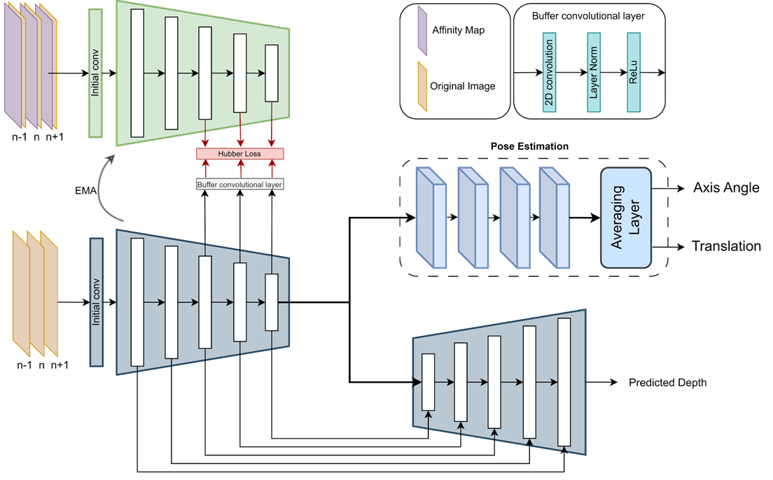
We utilize a student-teacher distillation mechanisms for this task. Teacher encoder (shaded green) is given the affinity information of each pixel in an input image along with the input image. Images below show a set of raw feature maps from the student and the teacher architectures. This shows how the affinity input changes the intermediate features of the teacher architecture promoting much sharper and detailed edges.

Our experiments have showns that directly distilling these raw teacher features into the student encoder can cause unstability in the training process and leads to poor performance. We have used a buffer convolutional layer between the teacher and student encoders to dampen the effects of distillation. Buffer layer contains 2 sets of convolutional layers with a kernel size of 3 and padding 1. Our experiments showed that using L2 loss for the distillation process can cause unstable training since small errors are also heavily penalized causing the network to overshoot frequently. L1 loss on the other hand does not penalize large errors enough for the model to converge.
We have decided to use Huber Loss for our knowledge distillation process, it applies L2 loss for larger errors and L1 loss for smaller errors resulting in a fast and smooth convergence.
Visual results below show how distilling affinity information into the student encoder has improved the prediction of depth around the corners.

Although our affinity distillation mechanism improves the depth prediction results for a large number of cases, it still is far from perfect. We notices certain cases where our mechanism seems to result in incorrect prediction at certain areas, especially around the edges. A few examples of such a case are shown below.

Around certain edges, the predicted depth seems to drop drastically which is inaccurate. Our future experiments would include using features from last 2 consecutive images to generate the depth mask for the current image, this approach has the potential to result in smoother results by reducing any inaccurate drop in depth score around the edges.